Creating an Absolute Reference

In earlier lessons we saw how cell references in formulas automatically adjust to new locations when the formula is pasted into different cells.
Sometimes, when you copy and paste a formula, you don't want one or more cell references to change. Absolute reference solves this problem. Absolute cell references in a formula always refer to the same cell or cell range in a formula. If a formula is copied to a different location, the absolute reference remains the same.
An absolute reference is designated in the formula by the addition of a dollar sign ($). It can precede the column reference or the row reference, or both. Examples of absolute referencing include:

$A$2	The column and the row do not change when copied.
A$2	The row does not change when copied.
$A2	The column does not change when copied.

To Create an Absolute Reference:

• Enter the numbers you want to calculate (e,g., 34,567 in cell B2 and 1,234 in cell B3).
• Then, create a simple formula (=B2+B3).

 

To create an absolute reference in the formula just created, insert a $ value before the B (column reference) and 2 (row reference) in the reference to B2 so the new formula reads, (=$B$2+B3)

 

Copy and Paste the formula to another adjacent cell. The formula now includes an absolute reference to B2, (=$B$2+D3).
 

 

Read more »

Revising Formulas

You can revise any formula that was previously written in a worksheet.

To Revise a Formula using the Keyboard:

• Double-click the cell that contains the formula you want to revise.
• The cursor can now move left and right between the values in the formula in cell B5.

 

• Make the necessary changes to the formula.
• Press the Enter key or click the Enter button to accept the new formula.

Read more »

Copy and Paste Formulas

The process to copy and paste a formula is identical to that process used to copy and paste text.

To Copy and Paste a Formula:

• Select the cell that contains the formula to be copied.
• Click the Copy button. Marching "ants" appear around the copied cell(s).

 

• Select the cell where the copied formula is to be pasted.
• Press the Enter key. The formula is copied to the new location.

Read more »

Filling Formulas to Other Cells

Sometimes, you will write a formula that gets used a lot in different places of a worksheet. For example, a spreadsheet may contain several columns of numbers. Each column will contain a formula that adds all the numbers in it. You could write the formula several times, once in each column. Or you could copy-and-paste it into each column. The fill formula method allows you to copy a formula and fill it into many different consecutive cells at the same time.
The mouse pointer changes to a black crosshair when passed over the fill handle, or the square box in the lower right corner of the cell.

 

To Use the Fill Handle to Copy a Formula to a Surrounding Cell:

• Click on the cell that contains the formula to be copied.
• Position the mouse pointer over the fill handle.
• Click and hold the left mouse button, and then drag the contents to the cell that's to receive the fill formula.
• Release the mouse button.
• Select the Copy Cells option in the fill formula drop-down menu.

 

The cell references in a formula are automatically updated when the formula is copied to other cells in the spreadsheet.
You can also use copy and paste to copy a formula to other cells. Click next to learn more about the copy and paste method.

Read more »

Creating Complex Formulas

Excel 2003 automatically follows a standard order of operations in a complex formula. If you want a certain portion of the formula to be calculated first, put it in parentheses.
If we wanted to add the contents of cell B2 and cell B3, for example, and then take that answer and multiply it by the data in cell A4, then we would need to define the following formula: =(B2+B3)*A4.

 

• Enter the numbers you want to calculate.
• Click the cell where you want the formula result to appear.
• Type the equal sign (=) to let Excel know a formula is being defined.
• Type an open parenthesis, or (
• Click on the first cell to be included in the formula (cell B2, for example).
• Type the addition sign (+) to let Excel know that an add operation is to be performed.
• Click on the second cell in the formula. The reference B3 displays where you want your result.
• End the B2+B3 operation by adding the close parenthesis, or )
• Type the next mathematical operator, or the multiplication symbol (*) to let Excel know that an multiply operation is to be performed.
• Click on the third cell to be included in the formula, cell A4.
• Very Important: Press Enter or click the Enter button on the Formula bar. This step ends the formula.

Try changing one of the values in the formula and watch the answer to the formula change.

Read more »

Complex Formulas Defined (continued)

Before moving on, let's explore some more formulas to make sure you understand the order of operations by which Excel calculates the answer.

5*3/2	Multiply 5*3 before performing the division operation because the multiplication sign comes before the division sign. The answer is 7.5.
5/3*2	Divide 5/3 before performing the multiplication operation because the division sign comes before the multiplication sign. The answer is 3.333333.
5/(3*2)	Perform the operation in parentheses (3*2) first and divide 5 by this result. The answer is 0.833333.
5+3-2	Add 5+3 before performing the subtraction operation because the addition sign comes before the subtraction sign. The answer is 6.
5-2+3	Subtract 5-2 before performing the addition operation because the subtaction sign comes before the addition sign. The answer is 6.
5-2*3	Multiply 2*3 before performing the subtraction operation because the multiplication sign is of a higher order than the subtaction sign. The answer is -1.
(5-2)*3	Perform the operation in parenthesis (5-2) first and then multiply by 3. The answer is 9.

Read more »

Complex Formulas Defined

Simple formulas have one mathematical operation. Complex formulas involve more than one mathematical operation.

The order of mathematical operations is very important. If you enter a formula that contains several operations--like adding, subtracting and dividing--Excel 2003 knows to work those operations in a specific order. The order of operations is:

1. Operations enclosed in parenthesis
2. Exponential calculations (to the power of)
3. Multiplication and division, whichever comes first
4. Addition and subtraction, whichever comes first

Using this order, let us see how the formula 120/(8-5)*4-2 is calculated in the following picture:

 

Let's take a look at another example:
2*(6-4) =?
Is the answer 8 or 4? Well, if you ignored the parentheses and calculated in the order in which the numbers appear, 2*6-4, you'd get the wrong answer, 8. You must follow the order of operations to get the correct answer.

To Calculate the Correct Answer:

• Calculate the operation in parenthesis (6-4), where the answer is 2.
• Multiply the answer obtained in step #1, which is 2, to the numeric 2* that opened the equation. In other words, multiply 2*2.
• The answer is 4.

When using formulas with cell references, the results change each time the numbers are edited.
Remember: In Excel, never do math "in your head" and type the answer in a cell where you would expect to have a formula calculate the answer.

Read more »

Creating Complex Formulas

Introduction

By the end of this lesson, learners should be able to:

• Create complex formulas
• Fill a formula to another cell
• Copy and paste a formula to another cell
• Revise a formula
• Create an absolute reference

Read more »

Challenge!

• Open your Monthly Budget file.
• Add cells C2 through C10 using a handheld calculator, the calculator on your computer, or pencil and paper.
• If you included additional monthly bills in cells C11 through 14, add cells C2 through C14 together to get your total monthly expenses.

How long did it take you to add all those numbers? Well, in the next three modules you will learn how Excel can do the math for you!

Type the total you came up with in cell C15.

Type a subtraction formula in C17 that subtracts the amount in C15 from the amount in C16.

Save and close the Monthly Budget file.

Read more »

Creating Simple Division Formulas

Creating division formulas is very similar to the addition, subtraction and multiplication formulas. To divide the contents of cell B2 by cell B3, you would need to insert a division operator / between them, =B2/B3.

To Create a Simple Formula that Divides One Cell by Another:

• Type the numbers you want to calculate in separate cells (for example, type 128 in cell B2 and 345 in cell B3).
• Click the cell where the answer will appear (B4, for example).
• Type the equal sign (=) to let Excel know a formula is being defined.
• Click on the first cell to be included in the formula (B2, for example).
• Type a mathematical operator (Ex: the division symbol /). The operator displays in the cell and Formula bar.
• Click on the next cell in the formula (B3, for example).
• If you include multiple cells in the formula, repeat steps 4 and 5 until the entire formula is entered.
• Very Important: Press Enter or click the Enter button on the Formula bar. This step ends the formula.

Read more »

Creating Simple Multiplication Formulas

Creating multiplication formulas is very similar to addition and subtraction formulas. To multiply two cells the formula, B2 and B3, you would need to insert a multiplication operator * between them, =B2*B3.

To Create a Simple Formula that Multiplies the Contents of Two Cells:

• Type the numbers you want to calculate in separate cells (for example, type 128 in cell B2 and 345 in cell B3).
• Click the cell where the answer will appear (B4, for example).
• Type =
• Click on the first cell to be included in the formula (B2, for example).
• Type a mathematical operator (Ex: the multiplication symbol *). The operator displays in the cell and Formula bar.
• Click on the next cell in the formula (B3, for example).
• If you include multiple cells in the formula, repeat steps 4 and 5 until the entire formula is entered.
• Press Enter or click the Enter button on the Formula bar to complete the formula.

Read more »

Creating a Simple Subtraction Formula Using the Point-and-Click Method

Formulas can be created by using either numbers or cell references in the definition. You can also use the mouse to select the cells to be used in the formula instead of typing the cell number or cell reference. Using this method, we are going to write a simple formula that subtracts one cell from another: =B3-B2.

To Create a Simple Formula using the Point and Click Method:

• Type the numbers you want to calculate in separate cells (for example, type 128 in cell B2 and 345 in cell B3).
• Click the cell where the answer will appear (B4, for example).
• Type the equal sign (=) to let Excel know a formula is being defined.
• Click on the first cell to be included in the formula (B3, for example).
• Type the subtraction sign (-) to let Excel know that a subtraction operation is to be performed.
• Click on the next cell in the formula (B2, for example).
• If you include multiple cells in the formula, repeat steps 4 and 5 until the entire formula is entered.
• Press Enter or click the Enter button on the Formula bar to complete the formula.

Read more »

Creating a Simple Addition Formula (continued)

But what if a column contains many numbers, each of which regularly changes? You don't want to write a new formula each time a number is changed. Luckily, Excel 2003 lets you include cell references in formulas.
A formula can add the value of two cells-B2 and B3, for example. Type any two values in these two cells and the formula will adjust the answer accordingly.
Using this method to calculate two numbers-128 and 345, for example-requires that you type 128 in cell B2, for example, and 345 in cell B3. The Excel formula, =B2+B3, would then be defined in cell B4.

To Create a Simple Formula that Adds the Contents of Two Cells:

• Type the numbers you want to calculate in separate cells (for example, type 128 in cell B2 and 345 in cell B3).
• Click the cell where the answer will appear (B4, for example).
• Type the equal sign (=) to let Excel know a formula is being defined.
• Type the cell number that contains the first number to be added (B2, for example).
• Type the addition sign (+) to let Excel know that an add operation is to be performed.
• Type the cell number that contains the first number to be added (B3, for example).
• Press Enter or click the Enter button on the Formula bar to complete the formula.

Read more »

Creating a Simple Addition Formula

A simple formula in Excel contains one mathematical operation only: one number plus a second number equals a third number. Writing a simple formula is really no more difficult than that: 1+1. The only difference in Excel is that all formulas must begin with the equal sign (=). It is not enough to type 1+1 in Excel because what will appear in the cell is "1+1." You must begin the equation with an equal sign, or =1+1. This holds true for any formula, simple or complicated, that adds, subtracts, multiplies or divides.
Let's add two numbers to create a third, 128+345=473. In Excel, this would be expressed by the formula, =128+345, as shown below.

To Create a Simple Formula that Adds Two Numbers:

• Click the cell where the formula will be defined.
• Type the equal sign (=) to let Excel know a formula is being defined.
• Type the first number to be added (128, for example)
• Type the addition sign (+) to let Excel know that an add operation is to be performed.
• Type the second number to be added (345, for example
• Press Enter or click the Enter button on the Formula bar to complete the formula.

Read more »

About Formulas

In school, you learned formulas used to calculate math problems. Microsoft Excel uses these same formulas to perform calculations in a spreadsheet.
A formula can be a combination of values (numbers or cell references) and math operators (+, -, /, *, =) into an algebraic expression. Excel requires every formula to begin with an equal sign (=).
The following table illustrates the mathematical operators learned in school and those represented in Excel 2003.

	School	Excel 2003
Addition	+	+
Subtraction	-	-
Multiplication	X	*
Division	/	/
Equals	=	=

The result of a formula-the answer to 2+3, for example-displays in the cell on the Excel worksheet. The formula is visible only in the formula bar. A formula's result will change as different numbers are entered into the cells included in the formula's definition.

Read more »

Creating Simple Formulas

Introduction

By the end of this lesson, learners should be able to:

• Understand the parts of an Excel formula
• Create a simple addition formula
• Create a simple subtraction formula using the Point-and-Click Method
• Create simple multiplication formulas
• Create simple division formulas

Read more »

Challenge!

• Open your Monthly Budget file.
• Type the following data in the spreadsheet:
  In cell A1, type Monthly Budget.
  In cell A2, type Rent or Mortgage.
  In cell A3, type Car Payment.
  In cell A4, type Cable.
  In cell A5, type Power.
  In cell A6, type Phone.
  In cell A7, type Insurance.
  In cell A8, type Credit Cards.
  In cell A9, type Groceries.
  In cell A10, type Gas.
• Type your other monthly bills in Column A, cells A11-A14 (if you have any).
• Type Total Monthly Expenses in cell A15.
• Type Income in cell A16.
• Type Savings in cell A17.

Save and close the Monthly Budget file.

Read more »

Selecting Multiple Cells

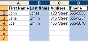
The currently-selected cell in Excel is called the active cell. You can also select a group of adjacent cells, or a cell range. Many operations can be done against a cell range: move it, copy, it, delete it or format it. A cell range can be defined in different ways: select a specific range of cells, select multiple columns or rows, or select the entire worksheet.

To Select a Range of Cells:

• Move to the first cell in the range.
• The mouse pointer becomes a large cross.
• Click-and-hold the left mouse button and drag left or right, up or down to the last cell you want to select.
• Release the mouse button.
• The cells you selected are shaded.

To Select All Cells in a Column or Row:

• Click the gray Column heading to select the entire column. (Click and drag the cursor across other column headings to select those columns).
  

Click the gray Row heading to select the entire row. (Click and drag the cursor down through the row headings select those rows).

To Select the Entire Worksheet:

• Click the gray rectangle in the upper left corner to select entire worksheet.
  

 

If the cells and columns you want to select are not directly next to one another, select one of the ranges you want to select, and hold down the Control key while selecting other ranges.

Read more »

Performing Undo and Redo

Sometimes, you might do something to a spreadsheet that you didn't mean to do, like type the wrong number in a cell. Excel 2003 allows you to undo an operation. Use the Undo button on the Standard toolbar to recover an error. The last single action is recoverable.

To Undo Recent Actions (typing, formatting, etc), One at a Time:

• Click the Undo button.

To Undo Several Recent Actions at Once:

• Click the arrow next to the Undo button.
• Select the desired Undo operation(s) from the list.

Microsoft Excel reverses the selected action and all actions that appear in the list above it.

An Undo operation can be cancelled by applying a Redo. This is useful when an Undo operation was mistakenly applied. Remember, a Redo is possible only if you have not changed an Excel spreadsheet since the last Undo operation was completed:

To Redo an Undo Operation:

• Press the Redo button.

To Redo several recent Undo actions at once:

• Click the arrow next to Redo button.
• Select the desired Redo operation from the list.
• Microsoft Excel reverses the Undo operation

Read more »

Deleting Information in a Cell

To Delete Data that Already Appears in a Cell:

• Click the cell that contains the information to be deleted.
• Press the Delete key, or
• Right-click and choose Clear Contents from the shortcut menu.
  

To Delete Data Being Typed But Not Yet Added to the Cell:

• Cancel an entry by pressing the Escape key.



Read more »